Welcome back to our series, Excel at Excel, by Steve Hughes! In his last post, Steve discussed using the Show Details feature. In this edition, he'll show you how to use the Flash Fill function by walking you through how to manipulate data and fill a column base using the Flash Fill function.
Flash Fill
Flash Fill is new functionality in Excel 2013 that allows you to manipulate data and fill a column based on actions you took. I like to think of it as somewhere between programming a macro and using the black cross to pull down formulas. I am going to illustrate a couple of ways to use this then you will have to take it from there.
First, you will need a set of data that this makes sense with. So let’s start with something obvious: You have a column of data that has a customer’s name formatted as Firstname Lastname. But you really need to format them as Last name, First name.
Here is the dataset we will use (it is the Indiana Hoosier players from the 80-81 season who were drafted):
| Year |
Round |
Pick |
Player |
NBA_Club |
Key |
| 1981 |
1 |
2 |
Isaiah Thomas |
Detroit Pistons |
1 |
| 1981 |
1 |
18 |
Ray Tolbert |
New Jersey Nets |
2 |
| 1981 |
5 |
115 |
Glen Grunwald |
Boston Celtics |
3 |
| 1981 |
8 |
180 |
Steve Risley |
Phoenix Suns |
4 |
| 1982 |
10 |
225 |
Landon Turner |
Boston Celtics |
5 |
| 1983 |
1 |
22 |
Randy Wittman |
Washington Bullets |
6 |
| 1983 |
2 |
40 |
Jim Thomas |
Indiana Pacers |
7 |
| 1983 |
2 |
41 |
Ted Kitchel |
Milwaukee Bucks |
8 |
| 1983 |
4 |
78 |
Steve Bouchie |
Detroit Pistons |
9 |
| 1983 |
7 |
141 |
Tony Brown |
Indiana Pacers |
10 |
In our first illustration, we will take the Player column and separate and reorder the name – Last name, First, name.
The Flash Fill function is located on the DATA tab as shown below:

Follow the next steps carefully to reproduce what I am doing:
- Highlight the Isaiah Thomas last name and copy it to an empty cell.
- Add a comma.
- Copy his first name over. This should have a column where you see, Thomas, Isaiah.
- Highlight the cell with the new value and click Flash Fill.
And you're done! You now have a column that is formatted the way you wanted it to be. Cool, huh?
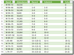
 The next set of data I am going to work with is the Hoosiers 2011-2012 season. The data includes a Record column which has the conference record part of the way through the set. What I want is to have separate columns for the overall and conference records.
This time I am going to select the cell on row 15 which has both records in it. The first column I will create will have the overall record. This is done by copying only the conference record over and flash filling the column - works great! The first row will have no data because the dash does not fit the pattern. The next column, I only copy the section in the parenthesis. However, this did not work. For the rows without a set of data in parenthesis, it copied that anyway. Let’s clear the column and try one other way.
After many attempts that did not  work, then next operation needed more patterns to follow. For rows 13 and 14, neither of which has a conference record, I placed an empty set of parenthesis (). Then for the conference record, I copied the conference record in parenthesis over. My results look like the table to the right. As you can see, it is pattern matching and sometimes it does not get you the results you would expect. However, it is a great tool and will get you most if not all of the way to the result you need with very little effort. Enjoy!
Have questions about Excel? Submit your questions in the section below and Steve will be more than happy to answer them!


-1.png)
Leave a comment